
Introducing PyBlackwell
Blackwell approachability, scalarization, and target sets as a control primitive.


A dashboard can hide a broken promise
Imagine watching a model climb a leaderboard. The number is moving in the right direction. The score is higher today than it was yesterday. It is easy to feel that the system has improved. But the score may be hiding a quiet bargain.
A model that is very helpful and very unsafe can look good under one weighting. A model that is safe but nearly useless can look good under another. The single number is not lying exactly. It is doing what we asked it to do: compressing two promises into one score.
For an AI assistant, that score might look like this:
score = w × helpfulness + (1 − w) × safety
The higher the value of w, the more the score rewards helpfulness. The lower the value, the more it rewards safety.
There are plenty of situations where such a tradeoff is legitimate. But it is a poor substitute for what you might call a contract, a set of promises that all have to hold at once. In many deployments, the requirement is not “make the weighted average look good.” It is closer to this:
average helpfulness ≥ 0.45
average safety ≥ 0.45
That is a different kind of object. It is not a line of algebra. It is a region in a plane.
In this case, the acceptable region is a rectangle. The model has to land inside it. A point above the safety threshold but below the helpfulness threshold fails. A point above the helpfulness threshold but below the safety threshold fails too. The question is no longer, “Which weight should we choose?” It is, “How do we move the long-run behavior of the system into the acceptable region, even when the world pushes back?”
That is the question PyBlackwell is built to explore.
The old theorem behind the new library
Blackwell approachability is a theory of repeated decision-making with vector payoffs. David Blackwell introduced it in 1956 for games where each round produces several payoff coordinates rather than one reward.
The setup is simple. The learner chooses an action. The environment chooses a response. The learner receives a payoff vector. The learner then tracks the running average of all payoff vectors seen so far. For the helpfulness-and-safety example, the target set is:
{(helpfulness, safety): helpfulness ≥ 0.45 and safety ≥ 0.45}
Blackwell called such a set approachable if the learner has a strategy that can force the running average toward it, no matter how the environment chooses its actions.
The standard strategy is geometric. When the running average is outside the target set, project it onto the set. The residual from the projection to the current average identifies the exposed violation. The learner then chooses a mixed action whose expected payoff lies on the safe side of the corresponding separating halfspace for every environment response.
The distinction is operational. The learner does not ask which action has the best blended score. It asks which action mixture repairs the currently exposed target-set violation. PyBlackwell implements that approach for finite vector-payoff games. Readers who want a deeper insight to Blackwell’s life and the approachability theorem can watch Rakesh Vohra's hour-long lecture at the Simons Institute.
What PyBlackwell provides
PyBlackwell is a Python library for finite vector-payoff games and target-set approachability experiments. It lets users define the game, define the target geometry, run Blackwell-style updates, and inspect the trace.
The library includes:
finite vector-payoff games through MatrixGame,
closed convex targets such as PointTarget, BoxTarget, OrthantTarget, PolytopeTarget, and composed/product targets,
solvers that choose mixed actions from target-set geometry,
convergence traces and certificates with distances, projections, halfspace residuals, minimax values, and backend warnings,
examples and command-line tools for target-set approachability, regret reductions, calibration, benchmarks, and trace summaries.
Optional features stay behind extras. Plotting uses the plot extra. Convex-optimization integrations live behind extras such as cvx. ML and RL adapters are separated from the core finite-game solver.
The final point is not the only output. A run can report the current average, its distance to the target, the projection used by the solver, the halfspace residuals, and any warnings from the numerical backend. For audits, that record usually carries more information than another reward curve.
Why target sets matter for ML
Many deployed ML systems are not single-metric systems. A deployed model may need to meet floors on helpfulness, safety, calibration, latency, and group-level behavior at the same time. A recommender may need to learn while keeping engagement, diversity, creator welfare, and safety within acceptable ranges. A forecasting system may need calibration, not just accuracy.
Scalarization is convenient because it turns a dashboard into one number. It also changes constraints into prices. Pricing is fine for tradeoffs the designer really wants to price. It is a poor fit for requirements that should not be bought away by gains elsewhere. Nor is the alternative just a pile of if statements. A rule such as “if safety is low, switch to the safer policy” can be useful as a guardrail, especially for hard per-request constraints. But it is not the same thing as a strategy for a repeated game. It does not ask how the environment will respond to the switch. It does not reason about mixtures of policies. It does not prove that the long-run average is being pushed back toward the target set. Blackwell’s algorithm uses the current violation as a game-theoretic signal: find the exposed direction, then choose a mixed action that prevents every environment response from making that violation worse in expectation.
Blackwell approachability fits requirements that can be written as: Keep the running average inside this acceptable set. Several ML problems can be written that way. Multi-objective reward floors become boxes or orthants. Calibration becomes a target where forecast discrepancies converge toward zero. External regret becomes the problem of approaching the nonpositive orthant of regret vectors. Fairness and distributional constraints can be written as residuals that should vanish or stay below limits.
Good candidates are systems where an aggregate score would hide the failure mode: safety evaluation, online decision systems, calibrated forecasting, multi-objective bandits, or audit-heavy deployments. In those settings, “the weighted score improved” is weaker than “the running average is inside the target set, and here is the residual certificate.”
A small world with three policies
The toy experiment is deliberately small. It is not meant to model a real product. It isolates one failure mode. Each round, the learner chooses one of three policies. The environment then chooses one of two contexts, benign or hard. The learner receives a two-dimensional payoff:
[helpfulness, safety]
The payoff table is:
The contract is the same rectangle as before:
average helpfulness ≥ 0.45
average safety ≥ 0.45
The environment is adversarial in a precise and limited way. It is a greedy one-step adversary. After the learner selects an action or mixed action, the environment chooses whichever context makes the next running average farthest from the contract region. It is not a worst-case-in-hindsight adversary, and it is not a learning adversary.
The distinction matters because “adversarial” does not mean “always choose the hard context.” The most damaging context depends on the learner’s action. Against balanced, the hard context hurts because helpfulness falls to 0.30. Against fast_but_unsafe, the benign context is worse because safety falls to 0.03 (benign gives (0.86, 0.03), distance ≈ 0.42; hard gives (0.73, 0.18), distance ≈ 0.27). The adversary is choosing distance from the box, not the context with the more alarming name.
The scalar baselines get a forgiving comparison. They sweep 21 weights from w = 0.00 to w = 1.00 in steps of 0.05:
score = w × helpfulness + (1 − w) × safety
The experiment then reports the best scalar weight after the fact. PyBlackwell does not choose a weight. It only receives the target set.
The run reaches the rectangle
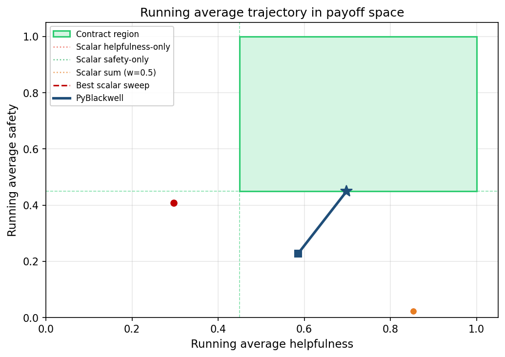
The green rectangle in Figure 1 is the contract region. A point inside it satisfies both floors. The PyBlackwell trajectory begins below the safety threshold. As the run continues, the average moves toward the rectangle. By the end, the star sits on the safety floor and inside the helpfulness interval. It is not deep inside the box, but it has reached the contract boundary to numerical tolerance. Mean final helpfulness across the seed-varied runs is about 0.704; mean final safety is 0.450.
The scalar baselines land outside the rectangle. The plot shows only two scalar markers because several rules collapse onto the same coordinates. Helpfulness-only and the w = 0.5 scalar sum both land on the orange high-helpfulness, unsafe point near (0.86, 0.03). Safety-only and the best scalar sweep both land on the red safer-but-not-helpful-enough point near (0.30, 0.42). The figure shows the core failure of scalarization in the experiment.
Distance rather than score
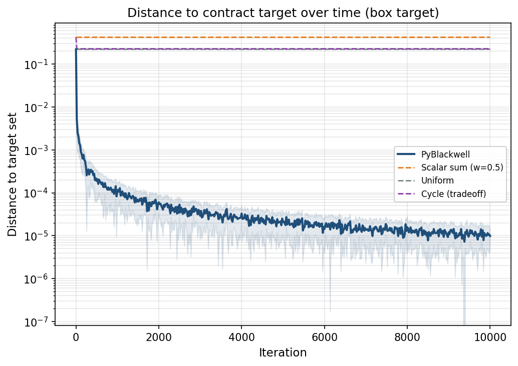
Figure 2 replaces the two payoff coordinates with a geometric diagnostic: distance to the target set. The vertical axis is logarithmic. The PyBlackwell curve drops and settles near zero. Across 20 seed-varied runs, its mean final distance is 9.8443 × 10⁻⁶
Uniform and cycle are simple non-scalar baselines. They miss mainly on safety, and their final distances are close enough that their curves are hard to separate by eye. The best scalar sweep is the most forgiving scalar comparison because it chooses the best weight after the run. It remains more than 0.15 away from the contract region.
The missing weight
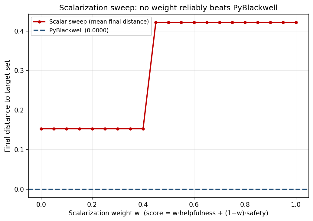
Figure 3 tests the obvious objection: maybe the scalar objective failed because the wrong weight was chosen. The sweep gives two plateaus and no usable middle. For w = 0.00 through w = 0.40, the scalar strategy chooses balanced. Against that policy, the greedy adversary chooses the hard context. Helpfulness falls to about 0.300, leaving a helpfulness shortfall of about 0.150.
For w = 0.45 through w = 1.00, the scalar strategy switches to fast_but_unsafe. Helpfulness now looks strong. The adversary switches too, for the reason shown in the payoff table: the benign context is farther from the box than the hard one because the safety violation is larger. The result is a safety shortfall of about 0.422. The step occurs between w = 0.40 and w = 0.45. Before the step, the scalar policy is too unhelpful. After the step, it is too unsafe.
No swept weight reaches the rectangle. PyBlackwell reaches the contract boundary to numerical tolerance; every scalar weight in the sweep stays outside. Numerically, the best scalar distance is 0.152752, while PyBlackwell’s mean final distance is 0.000009844. The relative reduction is about 99.99%, but the ratio is secondary. The categorical result is that one method reaches the contract and the other does not.
The endpoints
Across 20 seed-varied runs, PyBlackwell reaches the contract region: mean final helpfulness 0.704, mean final safety 0.450, mean final distance 0.0000, both shortfalls zero. The scalar baselines fall into two clusters. The best scalar sweep and the safety-only scalar both pick balanced and end near (0.300, 0.421) with a final distance of 0.1528. The w = 0.5 sum and the helpfulness-only scalar both pick fast_but_unsafe and end near (0.861, 0.028) with a final distance of 0.4219. Uniform and cycle are not duplicates of each other but land close, around (0.58, 0.23), at distances 0.2198 and 0.2254.
PyBlackwell also returns a certificate that the scalar baselines cannot produce. A representative certificate near iteration 10,000 of a single run reports a distance of 1.06 × 10⁻⁵, a running average of (0.698, 0.450), a projection point of (0.698, 0.450), a projection residual of (0.000, −1.06 × 10⁻⁵) computed as average minus projection, a minimax value of −6.03 × 10⁻⁸, halfspace residuals of (−6.03 × 10⁻⁸, −6.03 × 10⁻⁸), and no warnings. The negative minimax value and small halfspace residuals are consistent with satisfying the Blackwell halfspace condition; the projection residual has the same norm as the reported distance because of how it is computed. The certificate checks the geometry of the computation; it does not validate what “safety” or “helpfulness” mean.
Beyond the rectangle
The helpfulness-and-safety box is one target set among many. The same view applies to regret and calibration. The extended seed-varied run also tests PyBlackwell on two classical reductions: external regret and binary calibration. For external regret, where the target is the nonpositive orthant (no fixed action should look consistently better in hindsight), PyBlackwell’s mean final distance is 0.00362 against a best-baseline 0.531. For binary calibration, where the target is a zero discrepancy vector across forecast bins (when the model says “about 70%,” the empirical frequency should match), the numbers are 0.000228 against 0.000369. The calibration gap is narrower in both relative and absolute terms because simple baselines already remove most of the error, leaving less headroom. The same geometry handles all three examples: define the residual vector, define the acceptable set, monitor distance to that set.
It matters that the certificate in this experiment is a finite-game, full-vector-payoff certificate. In bandit or reinforcement-learning settings, PyBlackwell can still organize target-set diagnostics, but the guarantees need extra estimation, exploration, and concentration assumptions. The geometry carries over more directly than the theorem.
An even more interesting question lies beyond measurement. It is control. Where does an AI system face an environment that keeps changing in response to what the system does?
1. LLM deployment control
An LLM product already chooses among policies: different models, prompts, refusal thresholds, tool permissions, retrieval settings, moderation filters, rate limits, escalation paths, and human-review queues. The incoming prompt stream is not passive. Some users are ordinary. Some are adversarial. Recent safety work treats this as an adaptive problem: simple adaptive attacks can still bypass safety-aligned models, and AI-control work asks how control measures should scale as agents become more capable. See, for example, Andriushchenko et al. on adaptive jailbreaks and Korbak et al. on evaluating control measures for LLM agents.
Approachability would give the deployment layer a different shape. Instead of a static rule (“if the classifier says harmful, refuse”) the system would maintain a running vector of residuals. The controller would then choose a policy mixture that repairs the currently exposed violation. If unsafe completions accumulate, it may route more requests through stricter policies. If false refusals accumulate, it may relax or escalate differently. There is not yet a mature literature, as far as I can tell, on using Blackwell approachability as a live LLM deployment controller. For now, this is just an idea, it should be tested in practice, and it also carries risks. A controller that optimizes long-run averages may tolerate too many local failures. For LLMs, approachability should therefore be paired with hard per-request rules for non-negotiable harms.
2. Safe and multi-objective reinforcement learning
This is the area where Blackwell approachability already has the deepest connection to ML. For example Yu et al. study multi-objective competitive RL where performance is measured by the distance of the average return vector to a target set. Their paper makes explicit why the one-step repeated-game theorem is not enough for RL: in robotics, driving, games, and recommendation systems, decisions unfold over multiple time steps, and exploration becomes part of the approachability problem.
The contrast with standard constrained RL is useful. Constrained Markov decision processes often start from one main reward plus constraints. Lagrangian methods then attach multipliers to the constraints. That is powerful, but it still tends to convert the problem into a scalarized optimization loop. Safe-RL surveys describe a large family of such constrained and shielded methods, with safety during learning and deployment as the central issue. See Gu et al.’s safe-RL review.
Blackwell approachability starts from the vector contract instead. The “multiplier” is not fixed in advance. The policy can become nonstationary because the relevant objective changes with the accumulated state of the game. That can be better when the system must keep several long-run promises under disturbances or other agents.
3. Platform governance
Recommender systems and online platforms are repeated games. A platform recommends content. Users respond. Creators adapt. The next data set is shaped by those reactions. Klimashevskaia et al.’s work warns that recommender systems can produce reinforcement effects over time. It is also strategic. Creators change what they make. Users change what they click. A NeurIPS 2024 paper on user-creator feature dynamics shows how recommenders can influence both users and creators and can produce polarization and diversity loss.
Approachability could be useful here because the adversary need not be a malicious user. It can be the platform’s own feedback loop. If creator concentration rises, that becomes an exposed violation. If safety incidents rise, the exposed direction changes. If diversity is repaired at the cost of user value, the controller sees that too. The algorithm is not merely re-ranking by a weighted score, it is steering the platform’s long-run residual vector. There is some directly relevant approachability work, especially in fairness. Chzhen et al. adapt Blackwell approachability to fair online learning with unknown context distributions and instantiate it for group-wise no-regret, group-wise calibration, and demographic parity constraints.
My next paper
The research project I would like to write next is Blackwell approachability as an algorithmic primitive for adaptive AI systems. The thesis would say: “When an AI system faces a changing or strategic environment, target-set approachability can serve as a deployment-time and training-time control primitive for maintaining vector-valued contracts.” One of the experiments would test this idea in LLM deployment control. At each round, a defender would choose a mixed action over a small finite set of deployment configurations: refusal thresholds, system-prompt variants, classifier-ensemble weights, model-routing choices, or moderation settings. The defender would then observe a four-coordinate payoff: correct refusal on harmful prompts, helpfulness on benign prompts, calibration of the refusal classifier, and robustness to a held-out attacker. The contract would be a box with floors on all four coordinates. The primary metric would be distance to that contract region under attacks drawn from a public jailbreak benchmark such as JailbreakBench, which provides standardized attack artifacts, evaluation machinery, leaderboards, and a representative behavior dataset.
If the paper can prove that Blackwell approachability gives AI systems a mathematically clean way to react when the world pushes against one coordinate of a multi-objective contract, that makes it a candidate primitive for LLM routing, safe RL, online calibration, platform governance, and audit-heavy ML.